Physically, the most useful and interesting quantities that one seeks
to determine in quantifying upper atmospheric discharges are the
electric field ![]() and the electron distribution function
and the electron distribution function
![]() . As mentioned in Section 1.3, direct in
situ measurement of these or other quantities in the mesosphere and
lower ionosphere is rather difficult, as is remote sensing by means of
radar [Tsunoda et al., 1998].
. As mentioned in Section 1.3, direct in
situ measurement of these or other quantities in the mesosphere and
lower ionosphere is rather difficult, as is remote sensing by means of
radar [Tsunoda et al., 1998].
The intensity and spectrum of optical emissions from excited neutral
and ionized species depend on both ![]() and
and ![]() , providing
access to both of these quantities and others which can be derived
from them. In the following, we consider the factors affecting long
range passive optical remote sensing. A useful spectral emission line
should have a radiation lifetime as fast as the variations in electric
field due to a VLF pulse, for reasons discussed in
Section 1.3, and fast compared to the time scale for
relaxation of the electron distribution function . As it turns out, the
primary emissions from elves come from excited states with lifetimes
of
, providing
access to both of these quantities and others which can be derived
from them. In the following, we consider the factors affecting long
range passive optical remote sensing. A useful spectral emission line
should have a radiation lifetime as fast as the variations in electric
field due to a VLF pulse, for reasons discussed in
Section 1.3, and fast compared to the time scale for
relaxation of the electron distribution function . As it turns out, the
primary emissions from elves come from excited states with lifetimes
of ![]() 6
6 ![]() s and
s and ![]() 1
1 ![]() s (Section 2.4.3), while the
electron distribution thermalizes in
s (Section 2.4.3), while the
electron distribution thermalizes in ![]() 10
10 ![]() s.
s.
When enough natural signal is available, it is desirable to achieve
maximum spectral, as well as temporal, resolution. Spectra of
sprites have been measured
[Heavner, 2000; Mende et al., 1995; Hampton et al., 1996], but the limited
total optical output in elves is not conducive
to spectrophotometric measurements. More practical alternatives for
detecting a band of spectral lines such as
![]() are either to (1)
use very narrow optical filters to maximise the signal to noise ratio
obtainable from a single spectral line, or, if such a signal is
insufficient to overcome fundamental instrument noise or an adequately
narrow filter is not available, (2) a broadband filter may be used to
benefit from the extra signal available over several spectral lines of
a given molecular band. This latter strategy was pursued for high
time resolution photometry of elves, and more than one such filter is
used on different photometers to achieve at least some spectral
information. Section 3.3 treats the subject of
broadband photometric measurements.
are either to (1)
use very narrow optical filters to maximise the signal to noise ratio
obtainable from a single spectral line, or, if such a signal is
insufficient to overcome fundamental instrument noise or an adequately
narrow filter is not available, (2) a broadband filter may be used to
benefit from the extra signal available over several spectral lines of
a given molecular band. This latter strategy was pursued for high
time resolution photometry of elves, and more than one such filter is
used on different photometers to achieve at least some spectral
information. Section 3.3 treats the subject of
broadband photometric measurements.
In the following, we define the surface brightness which is used in all optical observations reported in this dissertation, and discuss the calibration of an instrument (such as the Fly's Eye) with a broadband optical response.
A photometer with an optical aperture ![]() and a field-of-view
subtending a solid angle
and a field-of-view
subtending a solid angle ![]()
![]() 1 responds to optical
emissions along its line of sight, as shown in Figure 3.5.
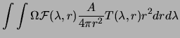
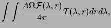
Let a unit volume of the optical source isotropically radiate photons
at rate
1 responds to optical
emissions along its line of sight, as shown in Figure 3.5.
Let a unit volume of the optical source isotropically radiate photons
at rate
![]() in the wavelength range
in the wavelength range ![]() to
to
![]() +
+![]() ; that is,
; that is,
 |
|||
 |
Thus the Rayleigh unit provides a measure which is convenient experimentally, via (3.3), and which relates easily via (3.1) to theoretical calculations determining volume emission rates in given molecular bands.
![\includegraphics[]{figures/spectralConsiderations.eps}](img268.png) |
We note for reference that to express a surface brightness in
W-cm![]() s
s![]() str
str![]() , we multiply the value in Rayleighs at wavelength
, we multiply the value in Rayleighs at wavelength
![]() by
by
![]() , where
, where ![]() and
and
![]() are the fundamental constants. We thus have,
are the fundamental constants. We thus have,
Photometric observations are reported as an apparent brightness,
without explicit knowledge or consideration of
![]() . In
addition, they typically represent measurements valid over a
restricted wavelength range, dependent on the sensor response range. In
contrast, theoretical calculations typically report emission
intensities integrated over an entire spectral band, based on
equation (3.1); for instance,
. In
addition, they typically represent measurements valid over a
restricted wavelength range, dependent on the sensor response range. In
contrast, theoretical calculations typically report emission
intensities integrated over an entire spectral band, based on
equation (3.1); for instance,
![]() spans the
wavelength range 575 nm to 2300 nm. An ideal instrument, with
spectral resolution, can thus instead provide a more fundamental
measure, the spectral surface brightness, given as
spans the
wavelength range 575 nm to 2300 nm. An ideal instrument, with
spectral resolution, can thus instead provide a more fundamental
measure, the spectral surface brightness, given as
A real photometer responds with a count rate somewhat less than that
given by equation (3.3), depending on the quantum
efficiency of the detector. The voltage response
![]() of a
photosensitive device, for instance the anode of a photomultiplier or
a pixel of an intensified CCD, is given by
of a
photosensitive device, for instance the anode of a photomultiplier or
a pixel of an intensified CCD, is given by
When making broadband optical measurements of a source whose optical
output may vary with wavelength, we cannot unambiguously determine the
optical intensity if the instrumental
![]() also
varies with wavelength. Thus to express experimental intensities based on (3.4) we assume that
also
varies with wavelength. Thus to express experimental intensities based on (3.4) we assume that
In summary, to calibrate a broadband photometer we must choose an
appropriate wavelength
![]() which dominates the integral in
(3.4), determine the calibration factor
which dominates the integral in
(3.4), determine the calibration factor
![]() for that wavelength, and determine the instrument gain
behavior (e.g. the value of
for that wavelength, and determine the instrument gain
behavior (e.g. the value of ![]() ) in order that a variety of
gains can be used in observations.
) in order that a variety of
gains can be used in observations.
The measure of optical intensity discussed above is used in this work
because, although not an accurate count of photon flux, it does not
require any assumptions about the optical spectrum under observation.
However, as can be seen from Figure 3.6, the
expected responses to sprite luminosity in our instrument are dominated
by narrow spectral ranges. For blue photometers sensitive to the
![]() band, the dominant wavelength region is near 375 to 400 nm and
is determined mostly by the competing factors of the atmospheric
transmission and the blue filter response. For red photometers, the
PMT (photocathode) response and the longpass red filter select a portion of the
band, the dominant wavelength region is near 375 to 400 nm and
is determined mostly by the competing factors of the atmospheric
transmission and the blue filter response. For red photometers, the
PMT (photocathode) response and the longpass red filter select a portion of the
![]() spectrum near 700 nm. The dominance of a narrow spectral region
in each photometer justifies the use of
equation (3.5) and endows the measure
spectrum near 700 nm. The dominance of a narrow spectral region
in each photometer justifies the use of
equation (3.5) and endows the measure
![]() with physical significance.
with physical significance.
![]() can be taken to be an
approximate measure of the true brightness near the dominant optical
wavelength
can be taken to be an
approximate measure of the true brightness near the dominant optical
wavelength
![]() .
.
A more direct experimental comparison with the theoretical surface
brightness of equation (3.1) can be
made if (1) one band strongly dominates the instrument response, (2)
its spectrum
![]() is known, and (3) the atmospheric
transmission
is known, and (3) the atmospheric
transmission
![]() is known.
is known.
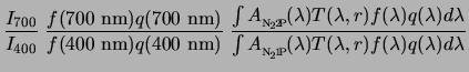
From these assumptions and equations (3.2),
(3.4), (3.5), and
(3.6), the total source brightness in band
![]() can be inferred from a wideband measurement:
can be inferred from a wideband measurement:
 |
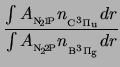
In a similar manner, the relative excitation rate of two bands can
be assessed through two-color photometry. For instance, the red and blue
optical filters shown in Figure 3.6 can
be used to assess the average excitation ratio of states
![]() and
and
![]() through their emissions in the
through their emissions in the
![]() and
and
![]() bands.
bands.
![\includegraphics[]{figures/opticalSource.eps}](img249.png)

![$\displaystyle \frac{V_{\rm obs}\ensuremath{G_{V_{{\rm H{(cal)}}}}}[A\Omega]_{\r...
...\rm obs} \: f(\ensuremath{{\lambda_0}})q(\ensuremath{{\lambda_0}})V_{\rm cal} }$](img291.png)
![$\displaystyle \alpha_{\ensuremath{{\lambda_0}}} \equiv \frac{ [A\Omega]_{\rm ca...
..._{\rm obs} f(\ensuremath{{\lambda_0}})q(\ensuremath{{\lambda_0}})V_{\rm cal} }.$](img296.png)